This article describes what pump curves and system are, why they are important, and how to use them for pump selection. If you don’t know what a pump curve is, start at the first section. If you’ve got some experience with pump curves, keep reading to found out more details on how to use them and their significance in chemical processes and water treatment.
Important: the pump curves we discuss below are ONLY relevant for centrifugal pumps. Don’t know what that means? See the glossary below!
Glossary
Before we start, a quick dictionary of words used in this article:
| Centrifugal pump | A pump with a direct connection between the inlet and outlet with an impeller (rotor) in the centre that adds energy to the fluid. The rotor does not force the fluid into or out of a chamber, but just adds two-directional energy to the fluid (centrifugal and forward). |
| Curve | The complete graph is called the pump curve. The line on the graph is the actual curve. |
| Gauge Pressure | The pressure at a given point relative to the surrounding atmospheric pressure, in other words the pressure difference between a system (like a pipe) and it’s surroundings. In practice this is simply the total absolute pressure minus the atmospheric pressure. |
| Head | A measure of pressure. Head is the total height to which a pump can raise water if it is going straight up. Imagine a long vertical pipe, with a pump connected to the bottom. The head of the pump (in meters or ft) is how high the pump can raise the water before it won’t go any higher due to the hydrostatic pressure at the bottom of the pipe. |
| Total Dynamic Head | TDH is the sum of the system head (how high the pump raises water from inlet to outlet) plus the hydrodynamic friction of the pipe. For pipe friction, see our article on this topic. |
| Impeller | A pump’s impeller is the rotating hub with curved vanes that adds energy to the fluid, similar to the one on a ship. |
Pump Curves – Definition
Very simply put, a pump curve shows how much liquid volume a pump can displace at a range of pressures. The two axes are the volumetric flow rate (in L/m, m3/hr, or other units) and the pressure (such as bar, psi, or kPa). The x-axis is normally used for flow rate, with the y-axis used for head (pressure).
System Pressure Explained
Imagine a long pipe that goes up a hill. To get the water to the top of the hill, you need to put in a certain amount of energy per liter of fluid, using the pump. If you turn the pump on and slowly increase the power output, nothing will happen at first because the pump isn’t adding enough energy and the impeller blades will just rotate without pushing the water away. At a certain point, the pump adds just enough energy to hold the fluid almost at the top of the hill but then it stops because gravity pulls on the water column. This is the Static Head of the system.
Now the pump power output increases more, and water starts to flow. This adds pipe friction to the equation, because of the inside of the pipe slowing down the water flow. The sum of pipe friction and static head is the Total Dynamic Head (TDH) of the system. The more water you pump through the system, the greater the pipe friction, and thus the greater the TDH becomes.
Pump Pressure Versus Flow Rate
This section explains the relation between system pressure and flow rate. If you understand this concept, just skip it!
A centrifugal pump at any given power setpoint has a direct and singular relationship between flow and pressure (head). Imagine a pump that is at maximum power and transfers water horizontally across a smooth pipe. There is no system pressure (TDH = 0) and the pump now pumps 50 m3/hr. Because the pipe ends up in the open air at atmospheric pressure, the pump outlet pressure is 0 bar gauge (see the Glossary for the definition of gauge pressure).
Now we slowly start to close a valve on the oulet pipe. The valve reduces the amount of water that passes through it and thus through the pump. Because the pump is still at maximum power output, the extra energy that is now not used to transfer water is converted to pressure. There is now a pressure differential between the inlet and the outlet of the pump. This pressure is the head of the centrifugal pump. With increasing system backpressure, e.g. due to more piping or equipment being added, the pump needs to use part of its energy to increase its outlet pressure. This reduces the flow rate it can pump water at.
Pump Curves Explained
Pump curves show the relationship between increasing pressure on the outlet of a pump, and the amount of water that can the pump can force through the system. Generally, higher backpressure (system pressure) means lower flowrate. This is normally a unique relationship, in which every backpressure (system pressure) only has one exact flowrate that can be pumped through the pump. See the pump curve below for a practical example.
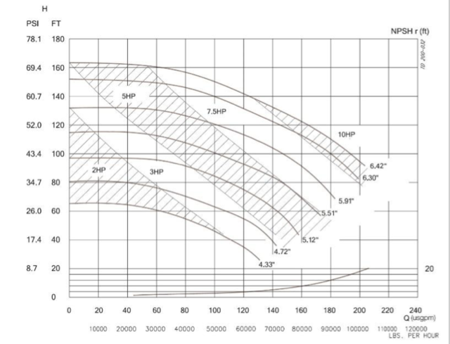
Image credit: Collaborativewriter, CC BY-SA 4.0 https://creativecommons.org/licenses/by-sa/4.0, via Wikimedia Commons, unchanged
The pump curve example above shows a typical pump curve for a medium size pump. The structure is as follows:
- Y-axis (left): The pump head i.e. the backpressure that the pump is pumping against. This is given in psi (pressure) and in ft (feet, height of the water column). Alternatively you could see the head in bar, kPa, MLc (meters of liquid column), and these can all be substituted for one another using the correct calculation (search our site for articles on this!)
- X-axis: the flowrate of the pump, indicated in US gallons per minute (usgpm) and Lbs (pounds) of water per hour. Both are useful depending on your system calculations. Modern pumps generally show this in cubic meters (m3) or liters, per hour or per minute (sometimes per second).
- Pump curves: the actual pump curves are the black lines from left to right, bending down. Each line is accompanied by a number (e.g. 4.33″) and this is the impeller trim size, i.e. the diameter of the impeller.
- Pump power zones: the diagonal zones (striped and clear) with the respective pump powers (e.g. 2HP, 2 horsepower) written in them. These indicate how much power input the pump has at a certain point. This is used only for pumps that have a variable power output (sometimes called variable horsepower pumps).
As can be seen, the black lines show the direct relationship between pressure and flow. As an example, have a look at the pump curve for a pump with impeller size 4.72″. When this pumps starts up against a closed valve there is zero flowrate, so all the energy is converted to pressure. The pressure at the outlet of the pump will be 34.7 psi (80 ft head), assuming zero inlet pressure.
If the valve is fully opened, the pump can supply just over 140 us gallons per minute, at a system pressure of around 15 psi (35 ft head).
Pay attention to the output power though, because to get this flowrate the pump power will need to be increased from 2HP to 3HP, to be in the correct power zone.
What is NPSH r?
The Y-axis on the left side of the graph shows the NPSH r, which means Net Positive Suction Head required. This is a bit of a complicated concept which we’ll describe very shortly here: NPSH is an indication of how much suction pressure can be applied to the water before it starts to evaporate. In simple terms: water can start to evaporate if the pressure drops too low. If a pump has a high flowrate and high power, it draws (sucks) the water into the pump inlet. This causes a local low pressure zone at the inlet of the pump, which can cause the water to start to evaporate. This can severely damage the pump.
To ensure this doesn’t happen, the pool or tank that the water is drawn from needs to be far enough from its boiling point (flash point) for the water not to form gas on its way to the pump. This pressure difference between the vapour pressure of the liquid and the current pressure is is normally expressed in meters (or feet) of head, hence the name Net Positive Suction Head – the Net Positive difference between the vapour pressure and the system pressure on the Suction side, expressed in meters (or feet) of Head. If these are equal, the liquid is at its boiling point.
The NPSHr is shown on the right-side Y-axis and the line that expresses it is the bottom part of the graph.
System Curves
So the pump curve is the first half of pump selection. Now we need to know what happens with the system pressure. When we pump liquid through a pipe and through equipment, the friction of the liquid against the system resists the flow, which shows in the form of pressure on the outlet of the pump. This pressure goes up when the flow increases, and is almost always a unique relationship between the flow and (back)pressure.
Pump Selection Using System Curve and Pump Curve
The system curve is normally a simple curve that is used to select the pumps. To make it, the pressure drop calculations through the pipes are added to the expected pressure drop in each piece of equipment, for different flows.
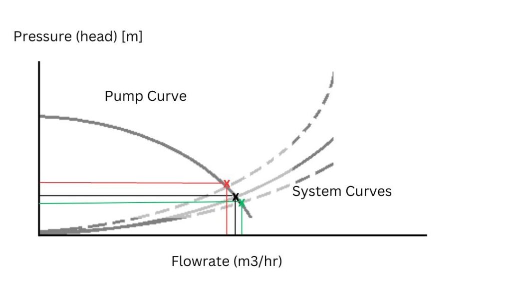
To select a suitable pump, it must be able to provide the correct flowrate at an acceptable system pressure. To do this, the pump curve and system curve are plotted in the same graph. The point where the lines intersect is the equilibrium point of the system, which dictates the flow and pressure of the system.
The diagram above also shows two dashed lines, one below and one above the main system curve. These are the system curves for when valves on the outlet of the pump are closed, restricting the flow and increasing the pressure on the outlet of the pump. Closing the outlet valve a little bit will result in lower flow and higher pressure on the pump outlet (the red ‘x’ on the left) and opening the outlet valve a little bit will result in a higher flow and lower pressure on the pump outlet (the green ‘x’ on the right).
Normally, for pump selection a system curve is used and plotted on a pump curve. Of course, it is not necessary to do it the graphical way, and calculations can also be used. This method, however, is a widely used method to visually assess the suitability of a pump for a given system, taking into consideration the flowrate and the pressure that the system requires.
Concluding Remarks
This article explains the basics of a pump curve, a system curve, and how to use the two to select a correct pump for a given system. This method is widely used for pump selection in water processing systems but also across other industries for pump selection. For more information, leave a comment or check out our other process engineering articles!
[…] High temperature: can impact the longevity of seals and the structural integrity of your casing and impeller, decrease bearing lifetime, and reduce NPSH-available (see this article if you don’t know what that means). […]